Modelling a Pandemic
So I recently had a student ask me about modelling he spread of disease using mathematics. He is going to do his EPQ on modelling zombie outbreaks and it looks really interesting. In preparation I had to dig back through my university notes and since I went through the effort I thought I'd talk about it here as well.
A common model used for this sort of thing is called an SIR model. The population is split into Susceptible (the healthy yet to get the disease), Infected and Removed (either people that have recovered and are now immune or those that have died. It is all one and the same to the model). Instead of talking about the total populations of the three groups, we tend to divide each by the total population to get the proportions of the population s(t), i(t) and r(t). I've written them all as a function of t because they will all change with respect to time. Because each is just the proportion of the total population we get that these three numbers should satisfy s(t)+i(t)+r(t)=1.
If we want to consider what will happen to the groups as time changes then we need to think about their derivatives with respect to time. The susceptible group is never going to increase, so its derivative is going to be negative, but we have to think about what it is proportional to. If there are more susceptible people then there are more people that are able to catch the disease. Also if there are more infected people walking around then there is also more chance of getting infected. So we can put this together with a constant of proportionality b for ds/dt=-bs(t)i(t)
Similarly the removed will grow proportional to how many infected people there are. So dr/dt=ki(t). The infected group has people dropping in from s(t) and dropping down to r(t) so we can get its differential equation by combining the rates from the other two. Here is our collection of differential equations so far:
ds/dt=-bs(t)i(t)
di/dt=bs(t)i(t)-ki(t)
dr/dt=ki(t)
The constants b and k we can choose to match the rate of whichever disease we are trying to model. Let's try a specific example: if each susceptible person has an encounter where they might catch the disease every two days and it takes about three days for the disease to either kill you or for you to recover then b and k are the reciprocals of these numbers so b=1/2 and k=1/3.
We also need some initial conditions. At the start almost everyone is susceptible and there is a very small part of the population which is infected. Let's pick some sensible numbers: s(0)=1, i(0)=10^-6, r(0)=0
Now we have a well posed problem of differential equations,, we want to know how each of our three dependent variables varies with time. There are ways to solve these explicitly, but they use quite sophisticated mathematics. Instead we are going to use a technique called Euler's Method to approximate the solution. The idea is to turn the problem from continuous into discrete. Each of the variables such as s(n) will be equal to value it was in the previous step, s(n-1) plus or minus some change. This change will depend on the size of the time step taken which we are going to called Δt.
Our equations become:
s(n)=s(n-1)-bs(n-1)i(n-1)Δt
i(n)=i(n-1)+(bs(n-1)i(n-1)-ki(n-1))Δt
r(n)=r(n-1)+ki(n-1)Δt
With the initial conditions the same as before s(0)=1, i(0)=10^-6 and r(0)=0. Δt can be chosen arbitrarily, so lets start at t=10 which means that our simulation will go in steps of 10 days at a time.
For instance the first step would give us:
s(1)=s(0)-bs(0)i(0)*10=1-1/2*1*10^-6*10=0.999995
i(1)=i(0)+(bs(0)i(0)-ki(0))*10=10^-6+(1/2*1*10^-6-1/3*10^-6)*10=2.6667*10^-6
r(1)=r(0)+ki(0)*10=0+1/3*10^-6*10=3.3333*10^-6
This represents what has happened 10 days in, but we can use these values to work out s(2), i(2) and r(2). This process is clearly quite time consuming to do manually so I popped them into a spreadsheet and automated the process. Going for 15 steps takes us to the end of day 150:
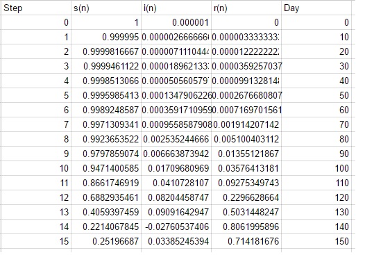
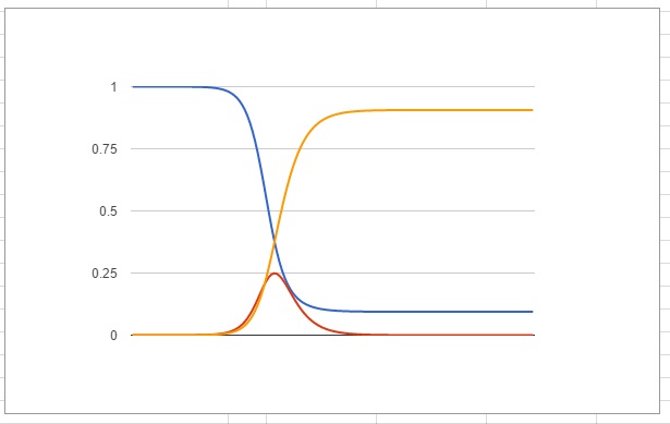
For this crude model let's have a look at what this looks like in graph form:
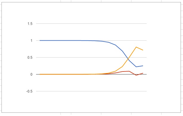
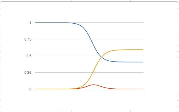
s is blue, i is red and r is yellow
Well that looks alright, we have the healthy population get infected at a faster and faster rate until it starts to lose steam until eventually the infection dies out. Some people never caught the disease, but most did. At any one time the number of infected people was never very high. However our graph is all jagged and the red line clearly goes below the axis at one point so the model isn't perfect. We can get around that by picking Δt to be a smaller step size. If I pick it to be 5 then I will have to do twice as many step calculations, but that is no problem since I can just drag down my formulae in the spreadsheet. So why not just go to Δt=1? Sure thing:

Again s is blue, i is red and r is yellow (2,3)
This looks a lot better and we can see our patterns clearly. Ok, earlier on we took the number of days until new contact with an infectious person as 2 and number of days until removed as 3. What happens when we play around with this?
(2,5)
This is what happens with the number days until you become immune or die is raised from 3 to 5. So (2,5). This brings everything forwards and it means that their is a higher peak of total number of infected people. The total number of susceptible people left at the end is far lower.
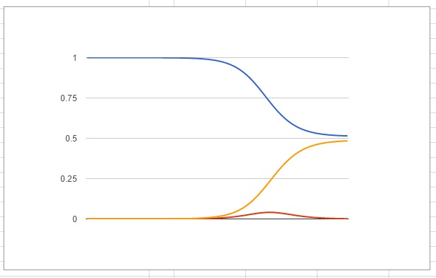
(2.2,3)
This one is very close to the original but with the first number changed from 2 to 2.2. This tiny change of 0.2 of a day makes it so that only half the population catches the disease rather than three quarters.
You can play around with these numbers for ages and get all sorts of results and there are lots of extensions to the SIR model, but for now I'll just leave you with the file.